Beef marbling measurement using spectral imaging: A multiple linear regression approach

Medición del marmoleado de carne de res usando imágenes espectrales: Un enfoque de regresión lineal múltiple

Victor Aredo^1, *; Lía Velásquez²; Nikol Siche³

¹Departamento de Operaciones Unitarias. Facultad de Química e Ingeniería Química, Universidad Nacional Mayor de San Marcos, Av. República de Venezuela s/n, Lima, Peru. varedot@unmsm.edu.pe

²Department of Food Engineering, Faculty of Animal Science and Food Engineering, University of São Paulo, Pirassununga, SP 13635-900, Brazil. lia.vc@usp.br

³Escuela de Ingeniería Zootecnista, Facultad de Ciencias Agropecuarias, Universidad Nacional de Trujillo, Av. Juan Pablo II s/n, Trujillo, Peru. nsichei@unitru.edu.pe

* Autor corresponsal: varedot@unmsm.edu.pe (V. Aredo).

ID ORCID de los autores

V. Aredo: https://orcid.org/0000-0002-3293-7696 L. Velásquez: https://orcid.org/0000-0001-8091-5611

N. Siche: https://orcid.org/0000-0002-7174-8337

ABSTRACT

This study aimed at measuring beef marbling scores in an objective and simple manner through spectral imaging and multiple linear regression (MLR). Beef marbling prediction by hyperspectral imaging and partial least squares regression (PLSR) was analyzed to calibrate and evaluate an MLR model with a few selected wavelengths. Data came from 44 beef samples and consisted of their spectral signatures (75 wavelengths) from hyperspectral reflectance images (400-1000 nm) and their marbling scores assigned by evaluators. The wavelengths that presented regression coefficients with the highest absolute values in the PLSR model, were used to calibrate the MLR model by a backward stepwise approach (p < 0.05). The coefficient of determination for prediction (R²_p) and the standard error of prediction (SEP) were evaluated. The MLR model was suitable for practical use because it required only 12 wavelengths for reliable predictions (R²_p = 0.824 > 0.8; SEP = 11.4% < 15%). A model is proposed for the objective and simple measurement of beef marbling score using multispectral imaging technology.

Keywords: hyperspectral imaging; partial least squares regression; predictive model; meat quality; multispectral imaging; multiple linear regression.

RESUMEN

Este estudio tuvo como objetivo medir el puntaje de marmoleado de carne de vacuno de una manera objetiva y sencilla mediante imágenes espectrales y regresión lineal múltiple (RLM). La predicción del marmoleado de la carne usando imágenes hiperespectrales y regresión de mínimos cuadrados parciales (RMCP), fue analizada para para calibrar y evaluar un modelo RLM con algunas longitudes de onda seleccionadas. Los datos provinieron de 44 muestras de carne de vacuno y consistieron en sus firmas espectrales (75 longitudes de onda) de imágenes de reflectancia hiperespectral (400-1000 nm) y las puntuaciones de marmoleado asignadas por los evaluadores. Las longitudes de onda que presentaron coeficientes de regresión con valores absolutos más altos en el modelo RMCP se utilizaron para calibrar el modelo RLM mediante un enfoque por pasos hacia atrás (p < 0,05). Se evaluaron el coeficiente de determinación de predicción (R²_p) y el error estándar de predicción (ESP). El modelo RLM era adecuado para uso práctico porque requería sólo 12 longitudes de onda para predicciones confiables (R²_p= 0,824 > 0,8; ESP = 11,4% < 15%). Se propone un modelo para la medición objetiva y sencilla del puntaje de marmoleado de carne de vacuno mediante tecnología de imágenes multiespectrales.

Palabras clave: imágenes hiperespectrales; regresión parcial de mínimos cuadrados; modelo predictivo; calidad de la carne; imágenes multiespectrales; regresión lineal múltiple.

Recibido: 24-09-2023.

Aceptado: 02-11-2023

Beef is one of the most consumed foods of animal origin. It is a source of high-biological value proteins and minerals, such as iron and zinc, vitamin A and B-complex vitamins (Liu et al., 2022; Vidal et al., 2022; Pereira & Vicente, 2013). Nowadays, beef production seeks to satisfy the demanding quality requirements of consumers. One of the quality attributes of interest to consumers is marbling, which consists of the amount and spatial distribution of intramuscular fat in the longissimus dorsi muscle (Gagaoua et al., 2022; Khaled et al., 2021). The consumers perceive this attribute as white specks or streaks in the lean muscle. Highly marbled steaks and other cuts of beef provide higher palatability (i.e., better sensory quality), which results in a higher marbling score (Khaled et al., 2021; Cheng et al., 2015).

Beef producers estimate or measure marbling as a reference to establish the commercial value of their product. The beef marbling is commonly measured manually using meat graders, which can be affected by the fatigue and natural subjectivity of the evaluator. In this context, several efforts have focused on developing marbling measurement methods using modern technologies, such as infrared spectroscopy, Raman spectroscopy, color computational imaging, and multi/hyperspectral imaging (Pinto et al., 2023; Echegaray et al., 2022; Cheng et al., 2015). Among them, multi/ hyperspectral imaging stands out since it combines digital imaging and spectroscopy, providing spatial and chemical spectral information about the samples (Jia et al., 2022; Özdoğan et al., 2021; Siche et al., 2016).

The high potential of multi/hyperspectral imaging to measure marbling and other quality attributes in the beef industry 4.0, is due to the application of data science strategies that handle the collinear and high-dimensional data to propose solutions with only the necessary data (Nychas et al., 2021; Echegaray et al., 2022). For measuring the beef marbling using multi/hyperspectral imaging, one strategy was to binarize sample images with a decision tree to determine fat area and subsequently apply a quadratic regression model to calculate beef marbling scores (Velásquez et al., 2017). Another strategy was to binarize images based on the maximum (fat/lean) ratio of gray value to determine the area of large, medium, and small fat particles and subsequently calculate meat marbling scores using a multiple linear regression (MLR) model (Li et al., 2011). In our previous study (Aredo et al., 2017), a partial least squares regression (PLSR) model was proposed to calculate beef marbling from the spectral signatures of the samples; considering procedural aspects, it can be affirmed that this model used a simple approach.

The solution to predictive tasks based on a calibrated PLSR model with full spectra can be simplified by calibrating an MLR model with selected spectral data (ElMasry et al., 2007). MLR models stand out for being easy to calibrate and understand for end users, which facilitates their practical application in industry through multi-spectral imaging technology (Su & Sun, 2018). In this sense, the present study explored measuring beef marbling scores by spectral imaging and MLR with a few selected wavelengths.

Data acquisition

This work used data from Aredo et al. (2017), where beef marbling score was predicted using hyperspectral imaging. Procedures and equipment for data acquisition and treatment, are briefly described here. A total of 58 beef samples (longissimus dorsi muscle) from Chachapoyas (Amazonas, Peru) were collected. These samples were divided into two sets: (1) a set of 44 samples for model calibration and (2) a set of 14 samples for prediction using the model.

The samples were scanned in a hyperspectral imaging system with a broom approach in reflectance mode. The hyperspectral imaging camera was a Pica XC model (Resonon Inc., USA), and the image acquisition/processing software was SpectrononPRO (Resonon Inc., USA). The system captured hyperspectral images in a spectral range of 400-1000 nm with a spectral resolution of 8 nm (i.e., 75 wavelengths were explored). The spectral signatures consisted of the average spectra in the region of interest from the hyperspectral images of each sample.

The reference measurement of the marbling score of the samples was made through the visual appraisal of 15 evaluators. It consisted of assigning scores by comparing photographs of the samples with the beef marbling standard of the Japan Meat Grading Association (JMGA, 2000), which ranges from 1 (minimum marbling) to 12 (maximum marbling).

Regression

The marbling scores of the samples assigned by evaluators were the dependent variable, while the spectral signature (75 wavelengths) of the samples was the dependent variable.

The calibration of the PLSR model by Aredo et al. (2017) for the prediction of beef marbling score using hyperspectral imaging was reviewed. PLSR is a machine learning technique introduced by Geladi & Kowalski (1986) used in chemometric tasks (Wold et al., 2001). It explains the descriptors by means of orthogonal factors, also called latent variables. The optimal number of latent variables is identified with the minimum mean squared prediction error value. Subsequently, the regression coefficients for the optimal number of latent variables are obtained.

Regression coefficients of PLSR models calibrated with near-ideal numbers of latent variables were also generated. This step was carried out with the intention of facilitating the identification of the wavelengths that carry important information for the prediction through the criterion of the highest local values of the regression coefficients.

The spectral signature of the samples was reduced considering the selected wavelengths. Using the reduced spectral signature and the marbling value assigned by the sample evaluators, a model was calibrated using multiple linear regression (MLR). This regression method is the most used when there is a linear relationship between the variables and is based on the principle of minimizing the prediction error (Çetin et al., 2022). In this work, this regression was used with the aim of a potential practical implementation of the simplified model through multispectral imaging technologies (Xie et al., 2018) and to facilitate intuitive recalibration for users with little mathematical / statistical / computational knowledge. For comparative purposes, a reduced PLSR model was calibrated with the same data used for the MLR model.

Calibration of the PLSR model was performed using Matlab 2023a software (MathWorks, Natick, MA, USA), while calibration of the MLR model was performed using MS Excel software (Microsoft INC). Both PLSR and MLR models, being linear models, can be represented by eq. (1) or by eq. (2) in detail.

(1)

In the case of the PLSR model, n: is the number of samples (44), k: is the number of wavelengths in the spectral signature (75), Y: is the response matrix (1 x 44) of marbling score values, β: is the matrix of regression coefficients (1 x 75), X: is the matrix of predictive variables constituted by the spectral signatures of the samples (75 x 44) and e: is the matrix of residual information not explained by the model (1 x 44).

In the case of the MLR and reduced PLSR models, n: is the number of samples (44), k: is the number of selected wavelengths identified from the analysis of the regression coefficients of the PLSR model, Y: is the response matrix (1 x 44) of marbling scores values, β: is the matrix of regression coefficients (1 x k), X: is the matrix of predictive variables constituted by the reduced spectral signatures (selected wavelengths) of the samples (k x 44) and e: is the matrix of unexplained residual information by template (1x44).

The performance of the models was evaluated in the calibration set using the coefficient of determination of calibration (R²_c) and standard error of calibration (SEC), and in the prediction set using the coefficient of determination of prediction (R²_p) and standard error of prediction (SEP) (ElMasry et al. 2007). The SEC and SEP are represented in eqs. (3-5).

(3)

(4)

(5)

where, Ŷ: is the predicted marbling score values; Y: the measured marbling score values; n_c: the number of samples (spectral signatures) in the calibration set (44); and n_p: number of samples (spectral signatures) in the prediction set (14) and the “bias”: is the systematic error.

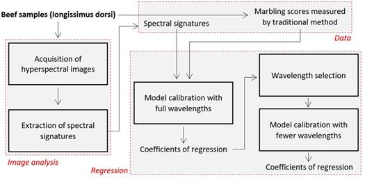
The figure 1 outlines the mentioned steps.

Full model verification

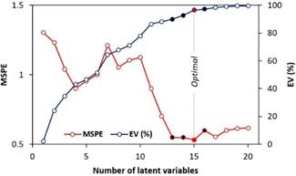
Verification of the calibration of the PLSR model by cross-validation (Figure 2) revealed that the ideal number of latent variables was 15, and that a similar number of latent variables (13, 14 and 16) can produce models with a low error level.

Gráfico, Gráfico de líneas

Descripción generada automáticamente

Figure 2. Mean Squared Prediction Error (MSPE) and Explained Variance (EV) in Partial Least Squares Regression (PLSR) models with different number of latent variables.

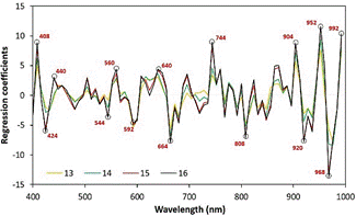
The analysis of regression coefficients of the PLSR model is commonly performed in the one calibrated with the optimal number of latent variables (15). However, as the PLSR models calibrated with 13, 14 and 16 latent variables present a low error, it was considered interesting to analyze the coefficients of these PLSR models together (Figure 3).

The remarkable overlapping of the regression coefficients provides evidence that the wavelengths that carry essential information for predicting marbling are similar to each other over the range of interest of the latent variables. Therefore, wavelengths with regression coefficients with higher absolute values should be useful for calibrating simplified models.

Figure 3. Coefficients of Partial Least Squares Regression (PLSR) models calibrated with 13-16 latent variables.

MLR calibration

The calibration of the MLR model (Table 1) using a stepwise procedure with a backward elimination approach revealed that the selected wavelengths that had the highest absolute values in the PLSR regression coefficient were significant (p < 0.003). The MLR model was statistically valid (p = 0.00) for predicting beef marbling (Table 1), and it has a predictive performance lower than the full PLSR model (Table 2), which is expected when less spectral information is used (from 75 to 12 wavelengths). On the other hand, the calibration of a PLSR model with the same reduced data and 12 latent variables yielded similar results to the MLR model (Table 2). Considering the simplicity, the MLR model is suitable for practical application because it achieves acceptable predictive performance (R²_p> 0.8, SEP < 15%) with reduced data (Siche et al., 2016; Su & Sun, 2018). 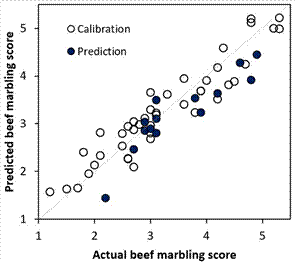In addition, the visual verification of the performance of the MLR model (Figure 4) indicates that it is adequate because both the calibration and prediction set points are close to the ideal line.

Table 1

Regression coefficients of the multiple linear regression model

Wavelength (nm)	Coefficients	Error	t-statistical	Significance
Interception	-3.898	1.711	-2.28	0.030
408	0.788	0.226	3.49	0.001
560	4.833	1.393	3.47	0.002
592	-9.330	1.710	-5.46	0.000
640	13.514	2.739	4.93	0.000
664	-12.589	2.428	-5.19	0.000
744	7.691	1.524	5.05	0.000
808	-6.475	1.166	-5.55	0.000
904	16.752	3.855	4.35	0.000
920	-14.094	4.143	-3.40	0.002
952	15.374	3.426	4.49	0.000
968	-22.576	3.508	-6.43	0.000
992	6.388	1.856	3.44	0.002

Analysis of variance: F_Cal=21.56 > F_Tab= 2.08, p = 0.00.

Table 2

Performance of models in predicting beef marbling score

Type of model	Number of wavelenghts	Calibration		Prediction
Type of model	Number of wavelenghts	R²_c	SEC	R²_p	SEP	SEP (%)
Full PLSR*	75	0.962	0.2	0.908	0.3	6.6
MLR	12	0.893	0.4	0.824	0.5	11.4
Simplified PLSR	12	0.891	0.4	0.819	0.5	11.6

PLSR: Partial Least Squares Regression, MLR: Multiple Linear Regression, R²_c: coefficient of determination for calibration, SEC: standard error of calibration, R²_p: coefficient of determination of prediction, SEP: standard error of prediction.

* Aredo et al (2017).

A point to highlight is the limitation of the model, as it is calibrated with samples with marbling scores between 1.2 and 5.3 (Figure 4); it cannot be used for reliable predictions in samples with marbling greater than 5.3. However, this does not rule out the possibility that the selected wavelengths (Table 1) are used as a reference in the recalibration of MLR models for multispectral systems with beef samples with different marbling without the need for extensive statistical knowledge of the user.

Figure 4. Actual vs. predicted beef marbling score using the reduced multiple linear regression model.

Regarding the selected wavelengths for beef marbling score measurement, it is worth mentioning that some of them are similar to those used in the evaluation of the composition of beef by near-infrared spectroscopy. It is well known that the visible region of the spectrum (400-700 nm) is related to the pigments in the samples. In this sense, pigments, such as oxymyoglobin and myoglobin, usually have strong absorption in this region (Alomar et al., 2003). Some reported wavelengths are the 430 nm wavelength called the Soret absorption band in the blue region of the spectrum due to the heme protein, which is attributed to trace amounts of hemoglobin in meat; and the 574 nm wavelength that is related to oxyhemoglobin absorption (Cozzolino & Murray, 2002). In near-infrared region, the wavelengths of 908 and 928 nm are attributed to proteins and fats, respectively (Alomar et al., 2003). Furthermore, the 970 nm wavelength is related to the second O-H stretching overtone due to the presence of water in the sample (Cozzolino & Murray, 2002; Alomar et al., 2003).

Complementary analyses

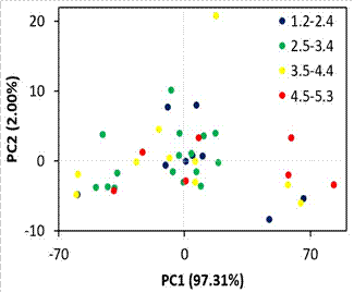
Principal component analysis revealed that 99.31% of the variance of the spectral data was captured with the first and second principal components (Figure 5 and Figure 6). In the score plot (Figure 5), it is not possible to differentiate samples with different beef marbling scores. It indicates that the high variance captured from the spectral data by the principal components does not necessarily imply class differentiation due to the unsupervised nature of the technique (Munera et al., 2018).

Figure 5. Scores plot (principal component 1 vs principal component 2) of spectral data of samples with different beef marbling scores.

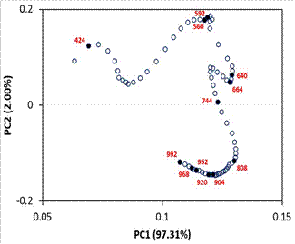
The loadings plot (Figure 6) revealed that the loadings of the wavelengths are positive in the first principal component, while part of the loadings are negative in the second principal component. The loadings appear to form a continuous “curve” with peaks, troughs, and inflection points. These elements could be used as a reference to suggest the selected wavelengths to predict the quality attribute of interest. However, in this case, with only this result, it is difficult to choose these wavelengths precisely.

The loadings plot including the wavelengths selected by multiple linear regression analysis (Figure 6), confirms that most of the selected wavelengths are in positions that define the “curve”. An interesting fact is that the selected wavelengths are “balanced” concerning the principal component 2; that is, six of them have positive values, and the other six have negative values. Moreover, the selected wavelengths have relatively high values in principal component 1, except for the 408 nm wavelength. This suggests that the selected wavelengths for predicting quality attributes can be confirmed with the loadings plot of principal component analysis.

Figure 6. Loadings plot (principal component 1 vs principal component 2) of spectral data of beef samples with different marbling scores*.

* Black points are the loadings of wavelengths used in multiple linear regression model.

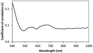
The evaluation of the correlation coefficient of each wavelength with actual beef marbling scores (Figure 7), revealed that all the wavelengths were weakly correlated with beef marbling scores. In this sense, this result cannot support the selection of wavelengths to calibrate simplified linear models (Aredo et al., 2019).

Gráfico, Gráfico de líneas

Descripción generada automáticamente Figure 7. Correlation coefficients (r) between each spectral wavelength with actual beef marbling scores.

Alomar, D., Gallo, C., Castaneda, M., & Fuchslocher, R. (2003). Chemical and discriminant analysis of bovine meat by near infrared reflectance spectroscopy (NIRS). Meat science, 63(4), 441-450. https://doi.org/10.1016/S0309-1740(02)00101-8

Aredo, V., Velásquez, L., & Siche, R. (2017). Prediction of beef marbling using hyperspectral imaging (HSI) and partial least squares regression (RMCP). Scientia Agropecuaria, 8(2), 169-174. http://dx.doi.org/10.17268/sci.agropecu.2017.02.09

Aredo, V., Velásquez, L., Carranza-Cabrera, J., & Siche, R. (2019). Predicting of the Quality Attributes of Orange Fruit Using Hyperspectral Images. Journal of food quality and hazards control, 6, 82-92. http://dx.doi.org/10.18502/jfqhc.6.3.1381

Çetin, N., Karaman, K., Kavuncuoğlu, E., Yıldırım, B., & Jahanbakhshi, A. (2022). Using hyperspectral imaging technology and machine learning algorithms for assessing internal quality parameters of apple fruits. Chemometrics and Intelligent Laboratory Systems, 230, 104650. https://doi.org/10.1016/j.chemolab.2022.104650

Bro, R., & Smilde, A. K. (2014). Principal component analysis. Analytical methods, 6(9), 2812-2831. https://doi.org/10.1039/C3AY41907J

Cheng, W., Cheng, J. H., Sun, D. W., & Pu, H. (2015). Marbling analysis for evaluating meat quality: Methods and techniques. Comprehensive Reviews in Food Science and Food Safety, 14(5), 523-535. https://doi.org/10.1111/1541-4337.12149

Cozzolino, D., & Murray, I. (2002). Effect of sample presentation and animal muscle species on the analysis of meat by near infrared reflectance spectroscopy. Journal of Near Infrared Spectroscopy, 10(1), 37-44.

Dong, J., Guo, W., Wang, Z., Liu, D., & Zhao, F. (2016). Nondestructive determination of soluble solids content of ‘Fuji’apples produced in different areas and bagged with different materials during ripening. Food Analytical Methods, 9, 1087-1095. https://doi.org/10.1007/s12161-015-0278-4

Echegaray, N., Hassoun, A., Jagtap, S., Tetteh-Caesar, M., Kumar, M., Tomasevic, I., ... , & Lorenzo, J. M. (2022). Meat 4.0: Principles and applications of Industry 4.0 technologies in the meat industry. Applied Sciences, 12(14), 6986. https://doi.org/10.3390/app12146986

ElMasry, G., Wang, N., ElSayed, A., & Ngadi, M. (2007). Hyperspectral imaging for nondestructive determination of some quality attributes for strawberry. Journal of food engineering, 81(1), 98-107. https://doi.org/10.1016/j.jfoodeng.2006.10.016

Gagaoua, M., Duffy, G., Álvarez García, C., Burgess, C., Hamill, R., Crofton, E. C., ... & Troy, D. (2022). Current research and emerging tools to improve fresh red meat quality. Irish Journal of Agricultural and Food Research, 61(1), 145-167. https://doi.org/10.15212/ijafr-2020-0141

Geladi, P., & Kowalski, B. R. (1986). Partial least-squares regression: a tutorial. Analytica chimica acta, 185, 1-17. https://doi.org/10.1016/0003-2670(86)80028-9

Jia, W., van Ruth, S., Scollan, N., & Koidis, A. (2022). Hyperspectral imaging (HSI) for meat quality evaluation across the supply chain: Current and future trends. Current Research in Food Science, 5, 1017-1027. https://doi.org/10.1016/j.crfs.2022.05.016

JMGA (Japan Meat Grading Association). (2000). Beef Carcass Grading Standards. Tokyo. Japan. Retrieved from http://wagyu.org/uploads/page/JMGA%20Meat%20Grading%20Brochure_english.pdf

Khaled, A. Y., Parrish, C. A., & Adedeji, A. 2021. Emerging nondestructive approaches for meat quality and safety evaluation—A review. Comprehensive Reviews in Food Science and Food Safety, 20(4), 3438-3463. https://doi.org/10.1111/1541-4337.12781

Khan, A., Munir, M. T., Yu, W., & Young, B. (2020). Wavelength selection for rapid identification of different particle size fractions of milk powder using hyperspectral imaging. Sensors, 20(16), 4645. https://doi.org/10.3390/s20164645

Li, Y., Shan, J., Peng, Y., & Gao, X. (2011). Nondestructive assessment of beef-marbling grade using hyperspectral imaging technology. In 2011 international conference on new technology of agricultural (pp. 779-783). IEEE. https://doi.org/10.1109/ICAE.2011.5943908

Liu, J., Ellies-Oury, M. P., Stoyanchev, T., & Hocquette, J. F. (2022). Consumer perception of beef quality and how to control, improve and predict it? Focus on eating quality. Foods, 11(12), 1732. https://doi.org/10.3390/foods11121732

Munera, S., Amigo, J. M., Aleixos, N., Talens, P., Cubero, S., & Blasco, J. (2018). Potential of VIS-NIR hyperspectral imaging and chemometric methods to identify similar cultivars of nectarine. Food Control, 86, 1-10. https://doi.org/10.1016/j.foodcont.2017.10.037

Nychas, G. J., Sims, E., Tsakanikas, P., & Mohareb, F. (2021). Data Science in the Food Industry. Annual Review of Biomedical Data Science, 4, 341-367. https://doi.org/10.1146/annurev-biodatasci-020221-123602

Özdoğan, G., Lin, X., & Sun, D. W. (2021). Rapid and noninvasive sensory analyses of food products by hyperspectral imaging: Recent application developments. Trends in Food Science & Technology, 111, 151-165. https://doi.org/10.1016/j.tifs.2021.02.044

Pereira, P. M. C. C., & Vicente, A. F. R. B. (2013). Meat nutritional composition and nutritive role in the human diet. Meat science, 93(3), 586-592. https://doi.org/10.1016/j.meatsci.2012.09.018

Pinto, D. L., Selli, A., Tulpan, D., Andrietta, L. T., Garbossa, P. L. M., Vander Voort, G., ... & Ventura, R. V. (2023). Image feature extraction via local binary patterns for marbling score classification in beef cattle using tree-based algorithms. Livestock Science, 267, 105152. https://doi.org/10.1016/j.livsci.2022.105152

Siche, R., Vejarano, R., Aredo, V., Velasquez, L., Saldana, E., & Quevedo, R. (2016). Evaluation of food quality and safety with hyperspectral imaging (HSI). Food Engineering Reviews, 8(3), 306-322. https://doi.org/10.1007/s12393-015-9137-8

Su, W. H., & Sun, D. W. (2018). Multispectral imaging for plant food quality analysis and visualization. Comprehensive reviews in food science and food safety, 17(1), 220-239. https://doi.org/10.1111/1541-4337.12317

Velásquez, L., Cruz-Tirado, J. P., Siche, R., & Quevedo, R. (2017). An application based on the decision tree to classify the marbling of beef by hyperspectral imaging. Meat Science, 133, 43-50. https://doi.org/10.1016/j.meatsci.2017.06.002

Vidal, P. O., Cardoso, R. D. C. V., Nunes, I. L., & Lima, W. K. D. S. (2022). Quality and Safety of Fresh Beef in Retail: A Review. Journal of Food Protection, 85(3), 435-447. https://doi.org/10.4315/JFP-21-294

Wold, S., Sjöström, M., & Eriksson, L. (2001). PLS-regression: a basic tool of chemometrics. Chemometrics and intelligent laboratory systems, 58(2), 109-130. https://doi.org/10.1016/S0169-7439(01)00155-1

Xie, C., Chu, B., & He, Y. (2018). Prediction of banana color and firmness using a novel wavelengths selection method of hyperspectral imaging. Food chemistry, 245, 132-140. https://doi.org/10.1016/j.foodchem.2017.10.079